personal blog of Gaurav Ramesh
The Engineering Behind Fast Analytics - Columnar Storage Explained
At OpenTable, my team builds a guest data platform that helps restaurant customers understand their diners through real-time analytics and segmentation dashboards. Coming from a traditional product development background, we naturally gravitated toward the tried-and-tested stack: React frontends communicating with Java backends via RESTful APIs, MongoDB for its scale and flexibility in data storage, and JSON for all data transmission over the wire. While this serves well for transactional applications like diner profiles and reservation systems, and is a decent start for the analytical journey, the model doesn't scale for that use case. It's not that it doesn't work, but it's not quite what it can be.
The performance bottlenecks at various parts of the stack motivated me to explore modern data systems, including columnar storage, streaming protocols, and the architectural patterns that enable high-performance analytics. I discovered that while incredible tools and technologies are built with backend and data engineers in mind, tooling for the JavaScript ecosystem - both NodeJS and browsers - seems limited. The realization took me from learning about data systems to working on a personal open-source project: a comprehensive toolkit for Nodejs and frontend web applications to build fast analytical applications (It's a work in progress, but more on that soon).
This post is part of a multi-part series documenting my journey - from theory to practice, from reading to building - and is a combination of technical deep-dives, personal learning logs, and efforts to build in public.
A Very Short History of Columnar Stores
The idea of storing data in columns is not new. It was considered to be first introduced comprehensively in 1985 by GP Copeland and SN Khoshafian. Their paper, "A decomposition storage model (DSM)"[1], proposed storing data in binary relations, pairing each attribute value with the record's identifier. This approach organized data by columns rather than rows, which they argued offered advantages in simplicity and retrieval performance for queries involving a subset of attributes, though it required more storage space overall.
MonetDB[2] implemented these ideas by 1999, becoming one of the first systems to embrace columnar architecture for analytical workloads and showcasing their effectiveness. C-Store[3], developed in the mid-2000s, marked another crucial milestone, and introduced advanced concepts explained further in the post that are now standards in modern columnar storage systems.
The late 2000s and early 2010s saw a rise in developments in this area, with projects like Apache Parquet[4] (influenced by Google's Dremel[5] paper) bringing columnar storage to the Hadoop ecosystem.
The Core Concept: Columnar vs. Row-Oriented Storage
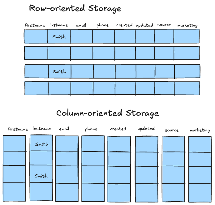
Traditional row-oriented databases store all data for a single entity together. The term row in a row-oriented system signifies the conceptual model of storing them, like a sentence written left to right in a notebook. In contrast, columnar data stores store data in columns, with each column containing values for a single attribute across all rows. This seemingly simple change has profound implications for analytical performance.
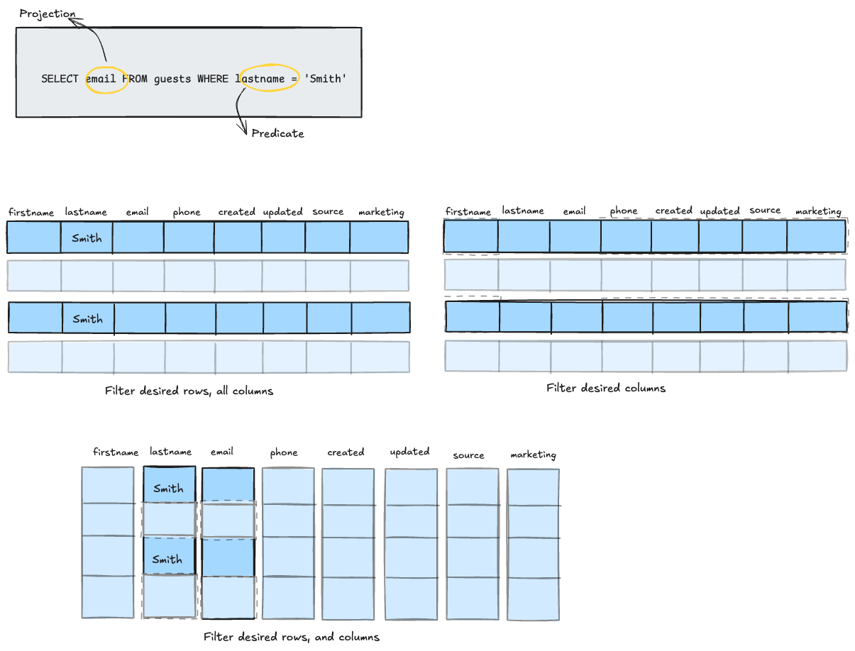
There are two key concepts to know when discussing transactional and analytical systems: predicates and projections. Predicates are the conditions by which you filter the entities(rows) you want(think of them as a WHERE clause in an SQL query). Projections are the fields(columns) that you want in the response(think of them as the column names you define in a SELECT statement).
If you think of your data as a list of rows, vertically stacked, predicates slice it horizontally, and projections slice it vertically. Transactional queries often rely on predicates to filter rows, with projections spanning the entire row, i.e. all the columns. Here's an example:
-- Example #1
SELECT * FROM order WHERE user_id = 1234;

-- Example #2
SELECT * FROM user WHERE user_id = 1234;
Projections in analytical queries involve a small subset of fields of the entity being queried. For example:
SELECT user id, name, num_orders FROM user_aggregates WHERE user_id = 1234Consider a table with 50 columns and millions of rows. In a row-oriented system, if you need only 3 columns, the database would still have to read all 50 columns for each row. With columnar storage, only the 3 relevant columns are accessed, massively reducing the I/O overhead, i.e. the amount of data you deal with while processing analytical queries.
Key Techniques Powering Columnar Stores
This idea of storing data in columns opens up new avenues for further optimizations. Here's a mental model to make sense of the following techniques: think of query execution as a pipeline that passes data through the various stages, potentially transforming it at each one. And it's a two-way pipeline at that: all the way from the client that wants the data to the system that computes and serves that data and back. In each direction, you can think of the places that benefit from optimization are: the network, CPU, memory and the disk.
In transactional systems(OLTP), the primary means of improving the performance of a query is indexing, which helps you get to the data you need faster, potentially all from memory. It's sufficient since you're usually dealing with one entity at a given point in transactional systems. But in analytical systems, you deal with a large volume of data in a given query, and hence reducing the data you work with in each stage of the pipeline is primarily how you get a better performance. The smaller the data you work with, the lower the cost, and the faster the pipeline.
Here are the primary ways of optimizing analytical pipelines. We'll look at each one of them in the post.
- Representing/encoding the data as efficiently as possible(data compression/column-specific compression),
- Filtering the data as much and as early as possible(column pruning, predicate pushdown),
- Expanding the data as late as possible(direct operation on compressed data, late materialization)
- Faster processing of the data(vectorized processing, efficient joins)
A word of caution - Although these are described as distinct techniques here, in reality, they are much more intertwined. The boundaries between where one ends and the others begin are not as clear and they often rely on each other for maximum gains.
Data Compression/Column-specific Compression
Columnar storage enables effective compression. Because data within a single column are of the same type and have similar characteristics, compression algorithms can achieve higher compression ratios. Techniques such as dictionary encoding, run-length encoding(RLE), bit packing, and delta encoding are commonly used in modern columnar stores.
Let's take an example to understand some of them - Say you have a data store for analyzing traffic on your website and are tracking the source from which a user entered your site. You might have noticed that when you click on a link in your email, the link usually opens up with a utm_source=email, or utm_source=newsletter, for example. The utm_source generally has a limited set of values that identifies the channel through which the user visited your site. The details of that source - domain, URL, time, cookies of the user - are tracked separately. Because each post or page could have thousands or millions of visits, your analytics database will have as many entries for each page, but with only a handful of values for the utm_source column.
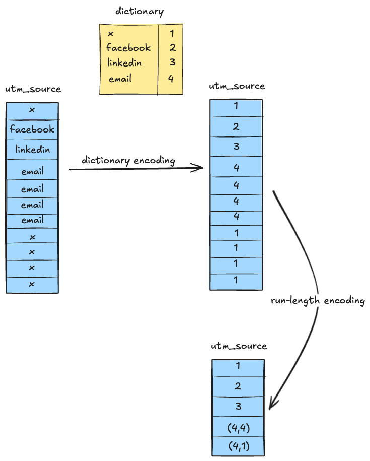
The string values of the source column can be dictionary encoded using integer values that pack tighter and are easier to work with(e.g. source email = 1, source twitter = 2, and so on.). Once that's done, if the consecutive entries in the DB have the same value, which could happen in instances like when you send out a campaign or a newsletter, it can be further compressed using run-length encoding. If a thousand consecutive entries have the same value for source, say 1, it can be stored as (1, 1000), rather than storing the same value a thousand times. Furthermore, if the integer representations take up less space than a 32-bit integer could hold, bit packing can compress it more, by reducing the number of bits needed to hold the value. In our case, if we have 200 different values for source, we only need 8 bits, rather than 32!
Column Pruning
One of the direct results of storing data in a columnar fashion is that it makes it easy to eliminate entire columns required(or rather, not required) for processing. Simply put, your query only ever touches the columns needed for the SELECT, WHERE, GROUP BY, ORDER BY or JOIN columns. Depending on the complexity of the query, you can eliminate a whole lot of data from even being brought into the query execution pipeline.
Consider a users table has 25 columns and the query is this:
SELECT first_name, last_name, email, phone FROM users WHERE num_orders > 10This query only needs 5 columns, so through column pruning we potentially reduce 80% of I/O overhead by eliminating the other 20 columns.
Predicate Pushdown
The idea behind predicate pushdown is to reduce the data footprint as close to the lowest possible level of execution as possible. Columnar stores do this by evaluating query predicates(think WHERE clause) at the storage layer thus removing the overhead of dealing with unnecessary data in memory and at the CPU. This becomes possible because columnar stores organize the data in blocks or chunks, with each block containing metadata about the range of values in the block(also called Zone Maps), like min/max values, null counts, and so on.
So when a query comes in, the metadata can be used to skip entire blocks. Only blocks that contain the matching data are selected to be read from the disk. Within the selected blocks, the filtering of specific values happens during decompression.
Example - Consider a simple query
SELECT name FROM users WHERE age > 50 AND city = 'New York'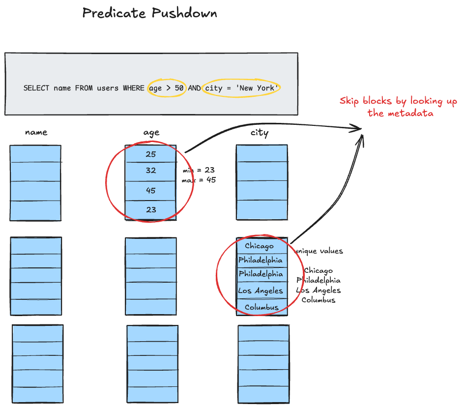
Without predicate pushdown, it'd read all column values for columns age and city, and then filter the data in memory. With predicate pushdown, it'd check block-level metadata for age and city columns, and skip blocks that have a max-age of 50, or those that don't have New York in the range of values within the block. For the remaining blocks, it'd apply the filter during decompression.
Direct Operation on Compressed Data
Storing data by columns also makes it easier to work on partially compressed data, which also reduces the I/O overhead. Consider a sample query
SELECT sum(salary) FROM employees WHERE department = 1002Now let's say that the data before compression looks something like this -
department: 1001, 1001, 1001, 1002, 1002, 1002, 1002, 1002, 1003, 1003
salary: 100000, 110000, 100000, 100000, 95000, 95000, 100000, 100000, 100000, 100000
After dictionary encoding and run-length encoding, department column might look like this
dictionary: {1001: 1, 1002: 2, 1003: 3}
department: 1, 1, 1, 2, 2, 2, 2, 2, 3, 3 (dictionary encoded)
department: (1, 3), (2, 5), (3, 2) (run-length encoded)
Similarly, salaries will look like this:
salary: (100000, 1), (110000, 1), (100000, 2), (95000, 2), (100000, 4)While evaluating the department predicate, the first three and the last two rows of the column can be skipped immediately merely by looking at the run-length encoded data(because they contain the departments that we're not interested in). The rows can then be encoded using a bitmap like 0001111100, where the 0s indicate the position of the rows that are to be excluded from the aggregation and the 1s indicate the rows that need to be included. Now the bitmap can be used to sum the salary column. The first two run-length encoded rows can be skipped. Since the next 5 rows need to be included, the third and the fourth blocks in salary can be multiplied right away, to get (100000 * 2 = 200000) and (95000 * 2 = 190000). The last block of salary needs to be expanded because only the first entry needs to be included out of the four, which gives us 100000. So the final sum is derived by adding three values rather than individually adding the salaries.
Late Materialization, aka Late Tuple Reconstruction
In the spirit of minimizing the data you work with that we alluded to earlier, the idea behind late materialization is that you expand the data only when you need to. While predicate pushdown lets us operate on just the data we want, based on the predicates in the query, late materialization delays the assembly of required projected fields until we have determined what rows need to be returned. This also reduces the overhead of processing unnecessary data at each stage.
Take the same query we considered in the predicate pushdown section
SELECT name FROM users WHERE age > 30 AND city = 'New York'We can work with age and city columns the entire pipeline up until we're ready to send the results back to the user, at which stage, we'll need to fetch the name column from the store.
Vectorized Processing
Vectorized processing in columnar databases operates on batches of data rather than individual values, leading to significant performance improvements.
SIMD(Single Instruction, Multiple Data) is a parallel processing technique invented to solve the problem of efficiently processing large arrays of similar data(mathematically called vectors) that require the same operation to be performed on each element. It's commonly found in most modern CPU architectures. Let's focus on the two main parts of the problem it solves -
- Large arrays of similar data - When data is stored by columns, this is exactly what you get while processing a single column
- Same operation to be performed on each element - This is true for most analytical queries, where you want to apply a predicate on the values of a specific column
Consider this query
SELECT sum(price) FROM sales WHERE user_id = 1234To find the desired rows, you're looking at the column user_id and performing the same operation, an equals check, on all the values in that column. In traditional processing you'd perform two things primarily sequentially -
- Check if value of
user_idcolumn of a given row is equal to1234 - If it is, add the value of the
sum - Repeat for the next row
With vectorized processing, chunks of data, say 1000 userid values at once is loaded into memory and compared to the value 1234 in parallel using SIMD. A bit of matches is then created to sum corresponding prices values in parallel.
Efficient Join Implementations
Columnar storage enables advanced join implementations beyond the traditional hash or merge joins. One example of such a technique is a semi-join, which aims to determine if one table has matching values in the join column of another table, without needing to return all column values from the second table. It uses bloom filters to achieve this. They are probabilistic data structures that help efficiently check for the potential existence of values, i.e. answer set membership queries. When asked whether a value exists in a set of values, they never produce false negatives(which means they can say with certainty that a value does not exist), but might produce false positives(which means they might say a value exists that does not). Instead of storing the actual join keys(which could be millions of values taking gigabytes), a bloom filter uses just a few megabytes to represent the same set with high accuracy.
Here's how it would work for a query like this
SELECT *
FROM orders o JOIN customers c ON o.customer_id = c.id
WHERE c.region = 'EMEA'
It filters customers by region column, say 10,000 out of a million customers. For the 10,000 customers, builds a bloom filter that only takes a few megabytes. Now it scans the orders table(say 100mn records), and tests each customer_id column against the bloom filter, skips the orders from customers that don't match, performs the more traditional and expensive hash joins on the remaining orders.
Conclusion
Combining all the above techniques, columnar data stores not only save storage space on the disk but also reduce I/O overhead, both of which result in cost savings for the organization. By working on lesser data and faster, they also offer significant performance gains for analytical workloads, and in a scalable manner. They have been gaining wide adoption in the areas of web analytics, business intelligence, machine learning infrastructure, log and event analysis, and real-time analytics, to name a few.
If you are a data practitioner who already works with columnar stores, I hope that the knowledge of the internals helps you squeeze the most juice out of them, and optimize them for your use cases. If you are an application developer building analytical products, think about your stack and consider introducing a columnar data store where you require performance and scalability. This post should help you make a case for why columnar storage might make sense for your needs. If you're an engineering leader considering adding a columnar datastore to your stack, knowledge of the above techniques should help you evaluate the trade-offs and make the right strategic decisions for your organization.
Resources
Share or Subscribe
Get notified when new posts are published. Once a month, I share thoughtful essays around the themes of personal growth, health & fitness, software, culture, engineering and leadership — all with an occassional philosophical angle.